📢
Announcement
Our existing VSTO has been renamed to Nasdaq Data Link Pro. This version is designed with better extraction, performance and stability.
Existing Users: If you are currently using the VSTO add-in, there is no action required on your part; you can continue to use the add-in as usual under the new name, Nasdaq Data Link Pro.

How to Use the Nasdaq Data Link Pro Excel Add-In

Click Get Data to access the Formula Builder dialog box.
Database: Select the database you would like to download from or search with a database code. (For instance, the database code for Retail Trading Activity Tracker is "RTAT".)
Data: Choose the table you would like to download.
Details: Use the tick boxes positioned at the top left of each column to select the columns you wish to include (by default, all columns will be downloaded). Use the filtering feature, symbolized by funnel icons situated at the top of each columns, to filter the data you wish to include (by default, all rows will be downloaded). Only columns designed as “filterable” in the database’s documentation page can be used as criteria to filter rows.
Placement: Select the cell where you would like to place the data. The “insert at cell” field will be updated according to your selection.
Click Import.

📘
NOTE:
If you are not receiving all the expected data, please double check your API key. If you can't find your products in the directory menu, try searching by product code. If a valid API key is not used, some tables will default to returning sample data.

How to Download Data Using the NASDAQ.TABLE Formula

In addition to the Formula Builder, the Excel add-in allows users to download tables data with the NASDAQ.TABLE formula. Users can directly type a formula into a cell to download data.

The structure of the formula is given below. Note that you can have multiple filters as part of a single query.

=NASDAQ.TABLE(Datatable code, columns, filter name, filter value, filter name, filter value)

	DESCRIPTION
Datatable code (required)	`DATATABLE CODE` Table codes can be found on each database page on our website. Example: The table code for Retail Trading Activity Tracker (“NDAQ/RTAT10”) can be found on data.nasdaq.com/databases/RTAT.
Filter columns (optional)	`COLUMN NAME` You can specify the column you wish to query here. If a column is not specified, all columns from the table will be retrieved. `{“COLUMN NAME”, “COLUMN NAME”}` To specify multiple columns, use curly brackets “{}” and indicate the columns you wish to query in quotation marks. Users are encouraged to directly reference cells that contain the column names. Examples: `ticker` retrieves only the data found in the column `ticker`. `A1:E1` retrieves the columns specified by these referenced cells.
Filter rows (optional)	By specifying one or more columns to act as the filter name, you can download your desired rows. If the value in a given column matches the specified filter value, the row containing that value is returned. Only columns designed as “filterable” in the database’s documentation page can be used as criteria to filter rows. Example: “date”, “ticker”, “activity”, "sentiment" are possible filters for the NDAQ/RTAT10 table.

DESCRIPTION

Datatable code (required)

DATATABLE CODE
Table codes can be found on each database page on our website.

Example: The table code for Retail Trading Activity Tracker (“NDAQ/RTAT10”) can be found on data.nasdaq.com/databases/RTAT.

Filter columns (optional)

COLUMN NAME
You can specify the column you wish to query here. If a column is not specified, all columns from the table will be retrieved.

{“COLUMN NAME”, “COLUMN NAME”}

To specify multiple columns, use curly brackets “{}” and indicate the columns you wish to query in quotation marks. Users are encouraged to directly reference cells that contain the column names.

Examples:
ticker retrieves only the data found in the column ticker.

A1:E1 retrieves the columns specified by these referenced cells.

Filter rows (optional)

By specifying one or more columns to act as the filter name, you can download your desired rows. If the value in a given column matches the specified filter value, the row containing that value is returned.

Only columns designed as “filterable” in the database’s documentation page can be used as criteria to filter rows.

Example: “date”, “ticker”, “activity”, "sentiment" are possible filters for the NDAQ/RTAT10 table.

Composition of a NASDAQ.TABLE Formula

The following NASDAQ.TABLE formula retrieves the complete history of revenue per share for Apple Inc. from the Retail Trading Activity Tracker (RTAT) table:

=NASDAQ.TABLE("NDAQ/RTAT10",{"date","ticker","sentiment"},"ticker","AAPL")

📘
NOTE:
Only columns designated as “filterable” in the table's documentation page can be used as criteria to filter rows.

We can break down this request as follows:

FORMULA COMPONENT	EXPLANATION
`=NASDAQ.TABLE("NDAQ/RTAT10",`	This portion of the call queries the NDAQ/RTAT10 table.
`{"date","ticker","sentiment"},`	This parameter will retrieve data only for the columns date, ticker and sentiment. If this portion is left blank then by default data for all columns will be returned.
`"ticker","AAPL"`	This filter removes everything except for where the ticker is AAPL

Using Filter Operators in the NASDAQ.TABLE Formula

The following are optional filter operators, which can be appended to all filters in your NASDAQ.TABLE formula, regardless of the table. The filter operators will further modify your results.

Filter	Description
.gt	Modifies the parameter to return values greater than the requested value
.lt	Modifies the parameter to return values less than the requested value
.gte	Modifies the parameter to return values greater than or equal to the requested value
.lte	Modifies the parameter to return values less than or equal to the requested value

Example 1: Query data after a specific date

The following NASDAQ.TABLE formula retrieves the sentiment for Apple Inc. where date is greater than or equal to 2012-01-01. Note the filter date.gte where the operator .gte (greater than or equal to) is appended to date.

=NASDAQ.TABLE("NDAQ/RTAT10",{"date","sentiment"},"date.gte","2012-01-01","ticker","AAPL")

Example 2: Query data for a specific date range

The following NASDAQ.TABLE formula retrieves the sentiment for Apple Inc. where date is greater than or equal to 2012-01-01 and less than or equal to 2022-01-01. Note the filter date.gte where the operator .gte (greater than or equal to) is appended to reportdate and note the filter date.lte where the operator .lte (less than or equal to) is appended to date.

=NASDAQ.TABLE("NDAQ/RTAT10",{"date","sentiment"},"date.gte","2012-01-01","date.lte","2022-01-01","ticker","AAPL")

Reference Cells in the Formula

Users are encouraged to directly reference cells that contain the desired specification when using the formula. The following two examples are meant to get you familiar with referencing cells in the Formula.

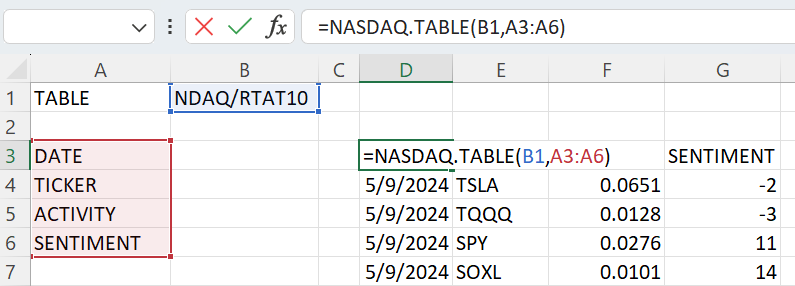
Example 1: Query multiple columns in tables

This example queries and downloads four columns from the NDAQ/RTAT10 table. Enter the Datatable Code (e.g., B1 cells) and column names you wish to query in the worksheet (e.g., A4, A5, A6, A7 cells). Use the NASDAQ.TABLE formula and reference these cells (e.g., A4:A7).

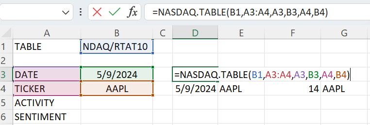
Example 2: Query multiple columns with filters in tables

This example queries and downloads four columns, filtering for only the AAPL value in the ticker column and for the 5/9/2024 value in the date column. To do this, enter the Datatable Code (e.g., B1 cells) and column names you wish to query in the worksheet (e.g., A3, A4, A5, A6 cells). Then enter the filter names and filter values you wish to filter by. Use the NASDAQ.TABLE formula and reference these cells.

📘
NOTE:
Support for QSERIES and QTABLE formulas have been deprecated.
QTABLE formulas have been replaced by NASDAQ.TABLE.
If you have existing worksheets built based on multiple QTABLE formulas, here is a simple guide to update your worksheets:

Open your Excel worksheet or workbook

Press Ctrl + F to open the Find and Replace dialog

If you intend to update the entire workbook, click "Option>>" to expand the dialog. Ensure "Within: Workbook" is selected to apply changes across all sheets.

In the "Find what" field, type 'Qtable'

In the "Replace with" field, type 'Nasdaq.table'

Click on "Replace All" to update all instances

Useful Links

For other useful tips on Excel add-in, please visit our FAQ portal.

For any questions, feedback or support request, please contact our client success team at [email protected].